Does a polynomial regression channel repaint?

A latest-window curve can revise older coordinates whenever it is refitted. A saved causal endpoint series can preserve each completed bar's original calculation with unchanged data and settings. Bar-close confirmation addresses developing inputs; it does not prevent later full-window redraws.

Which polynomial degree should I use?

Degree controls flexibility and the number of fitted parameters. Degree 1 is a straight line, degree 2 adds curvature, and degree 3 can change curvature within the window. Compare low degrees on held-out periods after specifying your decision rule; a smaller in-sample SSE does not establish better forecasts.

Why can degree 3 produce a wider band than degree 2?

The residual scale here divides SSE by N − degree − 1. Adding a parameter reduces that denominator. In the seven-price fixture, cubic SSE is lower, but its residual scale is 0.636209 versus 0.587570 for the quadratic.

Is a polynomial channel a 95% prediction interval?

No. A curve plus or minus two residual standard deviations is a descriptive channel. A statistical prediction interval needs additional uncertainty terms and justified error assumptions. Extending the curve outside its window adds extrapolation risk.

TradingView indicator research

Polynomial regression channels: degree, window and repainting

A polynomial regression channel fits a curve to a price window and offsets it by a chosen residual scale. Degree 1 is a line; degrees 2 and 3 allow curvature. The display rule matters as much as the degree: saving each completed bar's fitted endpoint creates a causal history, while redrawing the latest fitted curve can change older coordinates. Neither a close-confirmed curve nor a narrow band establishes forecast accuracy.

See the decision guide

See what an extra polynomial term changes

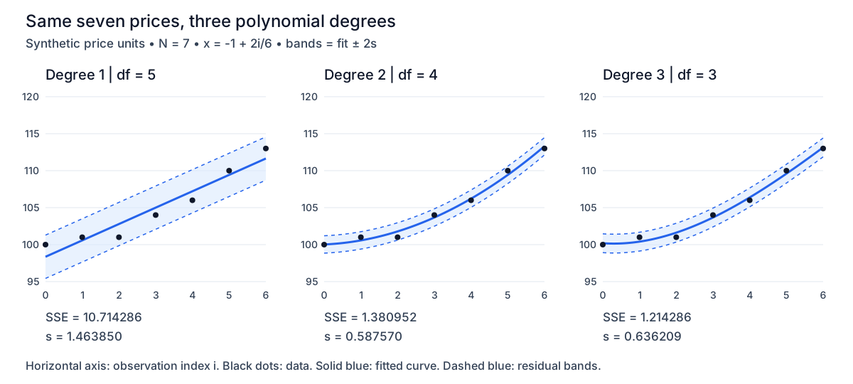
These original charts use seven synthetic prices: 100, 101, 101, 104, 106, 110 and 113, indexed 0 through 6. All three fits use exactly these observations and k = 2. Degree 3 reduces the sum of squared errors slightly relative to degree 2, yet its band is wider because one fewer residual degree of freedom remains. A tighter in-sample fit is not evidence of a better next-bar forecast.

Three original charts fit degrees 1, 2 and 3 to the same seven synthetic prices, with residual bands. The quadratic scale is 0.587570 and cubic scale is 0.636209 despite lower cubic SSE. — Synthetic arithmetic fixture, not market data. Dots show observations; solid curves show fits; dashed lines are fit ± 2s. All axes and bands use price units. View original source

Degree 1 estimates an intercept and slope. Degree 2 adds one curvature term. Degree 3 permits curvature to change sign inside the window; it also adds another estimated parameter.
A longer window changes which observations define the curve. It can span a different market regime; a shorter window leaves fewer observations per parameter. No window or degree is universally best.
The name does not identify one TradingView implementation. DonovanWall's original publication describes both full-window curves and endpoint bands. Check the author, source, width formula and display mode before comparing a community script with this example.

Normalize x and define the residual denominator

Let i = 0 denote the oldest observation and i = N − 1 the newest. Set x[i] = −1 + 2i/(N − 1), then fit yhat[i] = β0 + β1x[i] + … + βd x[i]^d by ordinary least squares. This is curved in x but linear in its d + 1 coefficients. Normalizing positions keeps the powers small; using raw timestamps or a large absolute bar_index is unnecessary.

NIST defines regression residual scale using N minus the number of fitted parameters. The channel here uses that scale descriptively. Interpreting it as an error-variance estimate requires a suitable regression model and error assumptions.
A band of ±2s is not automatically a 95% confidence or prediction interval. Regression intervals also account for leverage, uncertainty in the fitted mean and, for prediction, new-observation error. Financial residuals need not be independent or normally distributed.
NumPy's fitting documentation warns about high degree and poorly centered coordinates. Scaling x reduces a numerical problem; it does not remove overfitting, outliers, structural breaks or unstable behavior near window edges.

Quantity	Definition	Constraint or interpretation
Design matrix X	Row i is [1, x[i], …, x[i]^d]	Use distinct, equally spaced x values within each trailing window.
Coefficients	β = X⁺y, where X⁺ is the pseudoinverse	The example uses Pine matrix.pinv() on X, with degree capped at 3.
Residuals and SSE	e[i] = y[i] − yhat[i]; SSE = Σe[i]²	All residuals use one window's fitted curve, not separate rolling endpoint fits.
Residual scale s	sqrt(SSE / (N − p)), p = d + 1	The intercept counts as a parameter. Require N > p.
Channel	Lower(x) = yhat(x) − ks; Upper(x) = yhat(x) + ks	Constant vertical offsets in price units within a given fitted window.
Alternative residual RMS	sqrt(SSE / N)	A descriptive convention with a different denominator; do not compare it as the same s.

Recalculate the seven-price fixture

With normalized x = [−1, −2/3, −1/3, 0, 1/3, 2/3, 1], the quadratic is yhat = 311/3 + (93/14)x + 3x². Its fitted prices are [100.023810, 100.571429, 101.785714, 103.666667, 106.214286, 109.428571, 113.309524]. These displayed values are rounded; all residuals below use unrounded coefficients.

For degree 2, s = sqrt((29/21)/4) = 0.5875696514. At index 6, the k = 2 boundaries are 112.1343845067 and 114.4846631123.
The same quadratic has residual RMS sqrt((29/21)/7) = 0.4441609073. Dividing by 7 instead of 4 changes the band without changing the curve.
The quadratic residuals, in index order, are [−1/42, 3/7, −11/14, 1/3, −3/14, 4/7, −13/42]. Squaring and summing gives 29/21.
Independent exact-rational normal equations and a floating-point QR calculation reproduce the fixture. Across 24 additional constant and varying cases with degrees 1 to 3 and windows up to 100, fitted-value differences were below 5 × 10⁻¹³ price units. This verifies the numerical reference, not a live TradingView execution.

Degree	Coefficients β0, β1, β2, β3	SSE	Residual df	s	Newest fit
1	105, 93/14	75/7 = 10.714286	5	1.463850	111.642857
2	311/3, 93/14, 3	29/21 = 1.380952	4	0.587570	113.309524
3	311/3, 607/84, 3, −3/4	17/14 = 1.214286	3	0.636209	113.142857

Compare saved endpoints with a changing historical curve

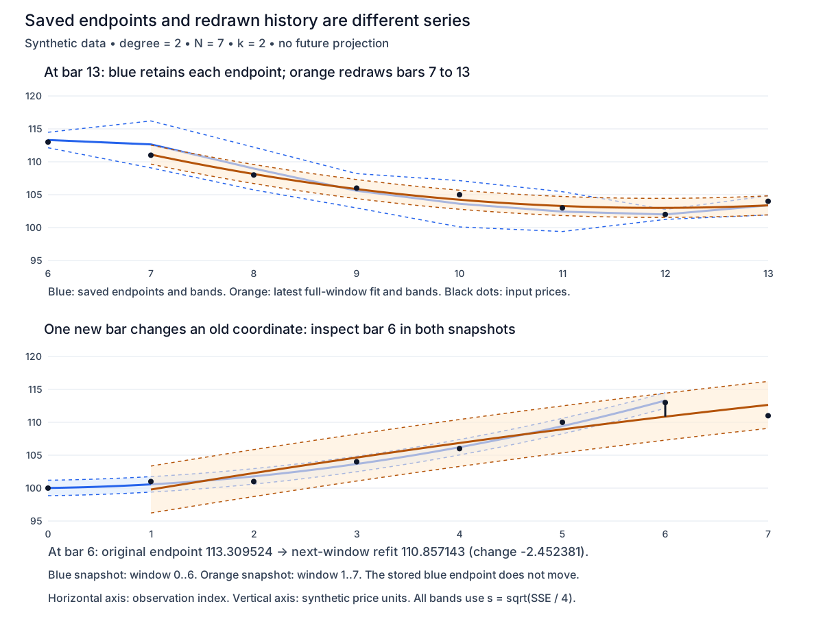
Extend the synthetic sequence to indices 0 through 13: [100, 101, 101, 104, 106, 110, 113, 111, 108, 106, 105, 103, 102, 104]. Keep N = 7 and degree = 2. Each blue endpoint uses only its own trailing window. The orange fit at index 13 uses prices 7 through 13 and evaluates that single curve across those older coordinates. The bottom comparison isolates the first roll from window 0..6 to window 1..7.

Original synthetic comparison. Saved quadratic endpoints at bars 6 to 13 differ from the latest full-window curve. In a second plot, bar 6 moves from 113.309524 under window 0 to 6 to 110.857143 under window 1 to 7. — Both plots are calculated from the printed 14-price fixture. Blue preserves the original calculation; orange evaluates a later window. Dashed boundaries use each fit's own residual scale. View original source

One added observation changes the displayed center at index 6 by −2.452381, although that historical price is still 113. The saved endpoint stays 113.309524. Comparing the latest redrawn line with an old candle cannot establish what a signal knew then.
At index 13, the latest curve puts index 7 at 111.095238. Index 7's original endpoint was 112.642857. The two series agree at index 13 because they share the same newest window, not because the earlier values are interchangeable.
Confirmation freezes the current input; it does not freeze a drawing that later code deletes and replaces. Separately, data-provider revisions or changed inputs can change recalculated history even for a causal endpoint implementation.

Same historical coordinate: index 6	Known when index 6 closed	Redrawn after index 7 closed
Window	0..6	1..7
Local x of index 6	1	2/3
Fitted center	113.309524	110.857143
Residual scale	0.587570	1.782855
Lower / upper at index 6	112.134385 / 114.484663	107.291433 / 114.422853
Close 113 versus center	Below	Above

Pine v6 example with both displays

This original implementation uses the public least-squares definition above. Blue plots expose completed-bar endpoint values. Orange line segments approximate the most recent completed window's fitted curve at bar positions and are replaced on the next completed bar. The orange drawing is descriptive and deliberately revises history; it supplies no backtest entries. The example contains no alerts, orders or forward extension.

For the fixture, enable "Use repeating 14-bar test fixture", keep Window = 7, Degree = 2 and Residual multiplier = 2. In TradingView's Data Window, Fixture index 6 should show endpoint 113.309524, SSE 1.380952 and scale 0.587570; index 7 should show endpoint 112.642857 and Previous coordinate in current fit 110.857143.
Fixture indices repeat every 14 loaded bars. Fits that would straddle a reset are suppressed; indices 0 through 5 have no channel with N = 7. This mode is an arithmetic test, not a price series or timestamp-stable signal; loading different chart history can shift its phase. Turn it off to use Source.
On an unfinished bar, the example shows no new endpoint and retains the preceding completed drawing. Invalid or missing windows clear the latest drawing at refresh and produce unavailable numeric outputs. The pseudoinverse is cached because X depends only on the input window and degree.

Pine Script v6. The final source passed the Pineify MCP syntax checker. Syntax success does not verify runtime chart behavior or trading performance.pine

//@version=6
indicator("Polynomial channel: endpoints and latest fit", overlay = true, max_bars_back = 100, max_lines_count = 500)
int n = input.int(7, "Window", minval = 3, maxval = 100)
int degree = input.int(2, "Degree", minval = 1, maxval = 3)
float k = input.float(2.0, "Residual multiplier", minval = 0.0)
float src = input.source(close, "Source")
bool fixture = input.bool(false, "Use repeating 14-bar test fixture")
bool drawWindow = input.bool(true, "Draw latest completed window")
if n <= degree + 1
    runtime.error("Window must exceed degree + 1 for positive residual degrees of freedom.")
if fixture and n > 14
    runtime.error("Test fixture requires Window <= 14.")
var array<float> samples = array.from(100.0, 101.0, 101.0, 104.0, 106.0, 110.0, 113.0, 111.0, 108.0, 106.0, 105.0, 103.0, 102.0, 104.0)
int phase = bar_index % 14
float y = fixture ? samples.get(phase) : src
int p = degree + 1
var matrix<float> design = matrix.new<float>(n, p, 0.0)
var matrix<float> pseudo = matrix.new<float>(p, n, 0.0)
if barstate.isfirst
    for i = 0 to n - 1
        float x = -1.0 + 2.0 * i / (n - 1)
        for j = 0 to degree
            design.set(i, j, math.pow(x, j))
    pseudo := design.pinv()

bool ready = bar_index >= n - 1 and (not fixture or phase >= n - 1)
for i = 0 to n - 1
    ready := ready and not na(y[i])
float center = na
float scale = na
float sse = na
matrix<float> fitted = matrix.new<float>(n, 1, na)
if ready
    // Center y to reduce cancellation for large price offsets.
    float base = y[n - 1]
    matrix<float> values = matrix.new<float>(n, 1, 0.0)
    for i = 0 to n - 1
        values.set(i, 0, y[n - 1 - i] - base)
    matrix<float> beta = pseudo.mult(values)
    fitted := design.mult(beta)
    sse := 0.0
    for i = 0 to n - 1
        float residual = values.get(i, 0) - fitted.get(i, 0)
        sse += residual * residual
        fitted.set(i, 0, fitted.get(i, 0) + base)
    center := fitted.get(n - 1, 0)
    scale := math.sqrt(sse / (n - p))

// Confirmed endpoint plots retain each bar's own trailing fit.
bool show = ready and barstate.isconfirmed
plot(show ? center : na, "Confirmed endpoint", color.blue, 2, plot.style_linebr)
upper = plot(show ? center + k * scale : na, "Endpoint upper", color.new(color.blue, 55), style = plot.style_linebr)
lower = plot(show ? center - k * scale : na, "Endpoint lower", color.new(color.blue, 55), style = plot.style_linebr)
fill(upper, lower, color.new(color.blue, 93))
plot(show ? sse : na, "Window SSE", display = display.data_window)
plot(show ? scale : na, "Residual scale", display = display.data_window)
plot(fixture ? phase : na, "Fixture index", display = display.data_window)
plot(fixture ? y : na, "Fixture value", display = display.data_window)
plot(show ? fitted.get(n - 2, 0) : na, "Previous coordinate in current fit", display = display.data_window)

// Orange drawing is replaced after each completed bar; it revises old coordinates.
var array<line> segments = array.new<line>()
bool refresh = barstate.islastconfirmedhistory or (barstate.islast and barstate.isconfirmed)
if refresh
    for segment in segments
        line.delete(segment)
    array.clear(segments)
    if drawWindow and show
        for i = 1 to n - 1
            int left = bar_index - n + i
            float a = fitted.get(i - 1, 0)
            float b = fitted.get(i, 0)
            array.push(segments, line.new(left, a, left + 1, b, color = color.orange, width = 2))
            array.push(segments, line.new(left, a + k * scale, left + 1, b + k * scale, color = color.orange, style = line.style_dashed))
            array.push(segments, line.new(left, a - k * scale, left + 1, b - k * scale, color = color.orange, style = line.style_dashed))

Test the boundaries before using the curve

The denominator and drawing behavior are part of the indicator's contract. A successful matrix operation alone is insufficient: a pseudoinverse can return coefficients for an underdetermined system, but that does not make its residual band meaningful.

For the first seven prices, evaluating the fitted polynomials at x = 2 gives 118.285714, 128.952381 and 124.119048 for degrees 1, 2 and 3. This is three bars beyond the fitted window, not an observed or predicted outcome. The disagreement illustrates degree sensitivity outside the data.
For a real-chart audit, save the script version, inputs, symbol, session, timeframe and values at a closed timestamp. Compare that same timestamp after several new bars and a reload. Record the endpoint plot separately from the latest-window drawing.
Any trading test needs explicit event timing, fills, exits, position sizing and costs. Use values available at the decision time; do not reconstruct trades from orange historical crossings.

Case	Expected behavior in this example
Shortest permitted window	N = d + 2: degree 1 needs 3 bars, degree 2 needs 4, degree 3 needs 5. Only one residual degree of freedom remains; this is a validity boundary, not a recommended trading setting.
N = d + 1	A full-rank polynomial can interpolate all observations, but residual df is zero. Reject the settings rather than dividing by zero or reporting a zero-risk band.
N < d + 1	Underdetermined fit; reject the settings. The UI also caps degree at 3 and window at 100.
Incomplete history or NA source	Return no fit until all N required observations are available. Never replace NA with zero or silently shorten the window.
Constant source	The constant is the fitted center and SSE = s = 0, so both bands coincide. The x matrix remains full rank.
k = 0	Both bands coincide with the fitted center even if residuals are nonzero.
Window edge or outlier	An incoming extreme price can bend the curve and widen its bands simultaneously. Test endpoint sensitivity, not just the appearance of the interior fit.
Extrapolation	No projection is drawn. Beyond x = 1, small coefficient changes can produce large differences; an offset band does not capture growing forecast uncertainty.

Give the coding agent a numerical acceptance case

Pineify's Pine Script AI Coding Agent can draft or revise a script from explicit formulas and requirements. Supply the normalized x convention, residual denominator, fixture and display rules above, and ask for source you can inspect. Request a syntax check, then compare the Data Window values and chart updates yourself.

Keep endpoint plots and full-window drawings separately labeled. If adding an alert, choose the confirmed endpoint threshold and retain the value that triggered it.
Use public formulas or source you have permission to use. This example is independently written; it does not reproduce a protected community indicator or promise numerical parity with one.

Where Pineify fits

Pine Script AI Coding Agent

Draft or revise a polynomial channel from explicit formulas, then request a syntax check and verify its values against the fixture. Review timing and chart behavior before adding trading rules.

Draft a polynomial channel

Related resources

TradingView indicator guides Linear regression channel formulas Causal and repainting kernel envelopes

Frequently asked questions

Educational calculation example, not investment advice. Prices and charts are synthetic and show no trading performance. Polynomial fits, narrow bands and confirmed values do not guarantee future prices or limit losses.

Sources and verification

Last verified: 2026-10-18

Published by Pineify. Pineify is an independent product and is not affiliated with TradingView. Sources support the technical explanations; examples do not establish trading performance.