Does heteroskedasticity make OLS coefficients biased?

Heteroskedasticity alone does not bias OLS coefficients when the conditional mean is correctly specified and the relevant exogeneity conditions hold. It changes their sampling variance and can invalidate ordinary standard errors. Omitted variables and future information are separate threats to the coefficient estimate.

Can I diagnose heteroskedasticity from raw return squares?

Raw return squares combine the conditional mean and variance. They can reveal changing magnitude, but a regression diagnosis should examine residuals from the specified mean model. A shifting mean can otherwise be mistaken for changing error variance.

Are HC3 standard errors enough for overlapping returns?

HC3 does not generally account for serial dependence caused by overlapping windows. Use a sampling design and covariance method that address that dependence, such as appropriately specified HAC inference. A larger HC3 standard error is not proof that overlap has been handled.

Are heteroskedasticity and heteroscedasticity different?

They are alternative spellings of the same property: nonconstant conditional error variance. Always specify the return model and conditioning information, since an unconditional volatility comparison can answer a different question.

TradingView Backtesting

Heteroskedastic Backtest Returns: Diagnostics and Consequences

Heteroskedasticity means the error variance of a specified return model changes with the conditioning information. It can invalidate ordinary regression standard errors without biasing OLS coefficients when the conditional mean is correctly specified and errors are exogenous. Inspect residuals after fitting that mean, compare variance across declared intervals, and use a covariance estimator that matches both variance changes and time dependence.

See the decision guide

Squared residuals expose a change that the fitted mean misses

The constructed example below has 12 equally spaced observations. Returns y are measured in percentage points and fitted to y = a + b × t, with t = 1 through 12. OLS gives a = 0.2 and b = 0.1. The second six residuals have four times the amplitude of the first six. This is an arithmetic demonstration, not market data or evidence that returns follow a time trend.

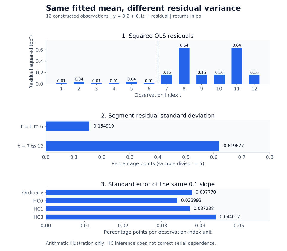
Constructed example: squared residuals rise from 0.01 or 0.04 to 0.16 or 0.64 squared percentage points; residual standard deviation rises from 0.154919 to 0.619677 percentage points; slope standard errors differ by covariance method. — Original calculation from the inputs in the next table. All panels use the same 12 observations; the split after observation 6 was specified when constructing the example. View original source

Within each six-observation segment the residual mean is zero. Descriptive sample variance uses Σ(e - segment mean)² / 5: 0.024 pp² in the first segment and 0.384 pp² in the second. Their square roots are 0.154919 pp and 0.619677 pp, a fourfold spread difference.
These are descriptive standard deviations of fitted residuals. The divisor 5 is not a claim that each segment provides an unbiased estimate of the underlying error variance after the full-sample regression.
Plot signed residuals against fitted values as well as squared residuals against time. Curvature or a level shift in signed residuals can indicate a deficient mean model. A variance chart alone cannot distinguish that problem from changing error variance.

t	Return y (pp)	Fitted y (pp)	Residual e (pp)	e² (pp²)
1	0.4	0.3	0.1	0.01
2	0.2	0.4	-0.2	0.04
3	0.6	0.5	0.1	0.01
4	0.7	0.6	0.1	0.01
5	0.5	0.7	-0.2	0.04
6	0.9	0.8	0.1	0.01
7	1.3	0.9	0.4	0.16
8	0.2	1.0	-0.8	0.64
9	1.5	1.1	0.4	0.16
10	1.6	1.2	0.4	0.16
11	0.5	1.3	-0.8	0.64
12	1.8	1.4	0.4	0.16

Reproduce the ordinary and robust standard errors

Keep the OLS coefficients fixed and change only their estimated covariance. With n = 12 and k = 2 fitted coefficients, the example has mean t = 6.5, Sxx = Σ(t - 6.5)² = 143 and SSE = Σe² = 2.04 pp². The ordinary slope standard error is √[(SSE / (n - k)) / Sxx] = 0.037770 pp per observation-index unit.

For this intercept-plus-one-regressor model, HC0 slope variance is Σ[(t - 6.5)²e²] / Sxx². HC1 multiplies that variance by n / (n - k) = 1.2. Apply the factor to the variance before taking its square root.
Leverage is hᵢ = 1/n + (tᵢ - 6.5)²/Sxx. HC3 replaces eᵢ² in the HC0 numerator with eᵢ²/(1 - hᵢ)². It gives additional weight to observations whose fitted residuals are reduced by high leverage.
The ratios are displayed for reproducibility, not as significance decisions. Twelve deliberately patterned observations do not justify treating these values as well-calibrated t tests. HC3 is larger here, while HC1 is smaller than the ordinary SE. Robust does not mean always larger.
None of these covariance choices changes fitted returns or the slope estimate. If omitted predictors, lookahead information or an incorrect mean model bias the coefficient, changing its standard error does not repair the estimate.

Covariance method	Slope estimate	Slope SE	Estimate / SE
Ordinary OLS	0.100000	0.037770	2.64760
HC0	0.100000	0.033993	2.94174
HC1	0.100000	0.037238	2.68543
HC3	0.100000	0.044012	2.27210

Use a Breusch-Pagan test with an explicit alternative

A Breusch-Pagan diagnostic asks whether error variance depends on selected explanatory variables. Specify those variables before looking for a favorable result. For this example, an auxiliary regression of e² on an intercept and an indicator for t > 6 compares the two declared segments. It is a variance diagnostic for that alternative, not a test of every possible variance pattern.

For the studentized Koenker version, the auxiliary regression gives R² = 0.466805, so LM = nR² = 5.601660. The asymptotic reference has one chi-square degree of freedom because there is one nonconstant variance regressor. The coefficient count in this auxiliary model is distinct from k = 2 in the mean regression.
Statsmodels uses the Koenker version by default with robust=True; the original Breusch-Pagan version uses a normal-error assumption. The studentized version relaxes that distributional assumption, but its usual calibration still requires an appropriate independent-error setting under the null. It is not an automatic correction for time-series dependence.
Do not interpret the numerical LM example as a reliable p-value for these 12 constructed observations. Small samples, outliers, chosen-after-the-fact splits and repeated testing can distort conclusions. Record the test variant, variance regressors, sample size and exclusions with any reported result.
A rejection does not identify the cause or prove a trading rule is useful. Failure to reject does not prove constant variance: the chosen alternative may miss the pattern, or the test may have little power.

Choose HC, HAC or a different model for the problem you have

Conditional mean, conditional variance and serial dependence are different properties. Volatility clustering can occur with uncorrelated signed returns, while overlapping return windows can create serial correlation even without a variance break. Inspect the ordered residuals and the sampling design before selecting inference methods.

Newey-West HAC incorporates lagged covariance terms as well as changing variance. The usual single-series implementation assumes consecutive, equally spaced periods. Report the maximum lag and kernel; compare reasonable bandwidth choices instead of selecting the one that produces significance.
The constructed residual pattern above also has time structure. Its HC comparison demonstrates arithmetic only. It does not establish that HC inference is sufficient for those observations.
If the goal is a volatility forecast or risk-scaled position size, HC and HAC standard errors are not that forecast. They estimate uncertainty in coefficients. A conditional-variance model has a different target and needs separate validation.

Observed issue	Relevant response	What it does not establish
Systematic signed residual pattern	Revisit the conditional mean, timing and omitted variables.	A robust covariance estimate does not remove coefficient bias.
Unequal error variance without material score autocorrelation	Use an appropriate HC covariance estimator; document HC0, HC1 or HC3.	HC does not make residual variance constant or validate the trading idea.
Heteroskedasticity and serial dependence	Consider HAC inference on a suitably ordered series; declare lag bandwidth, kernel and correction.	HAC does not cure nonstationarity, lookahead or arbitrary long-memory dependence.
A credible model of conditional variance	Consider variance modeling or weighted estimation with justified weights.	Estimated weights can be wrong; fit and validate them without future data.

Build the return dataset before testing a TradingView strategy

Choose the dependent variable first: asset returns, regularly sampled account returns, or trade-level outcomes. Account returns require dated equity valuations that include open positions and a defined cash-flow policy. Closed-trade P&L percentages occur at irregular times and use different capital exposure; they are not interchangeable with daily account returns.

For regular returns, preserve the valuation calendar, symbol, timeframe, session, costs, benchmark alignment and strategy version. Check missing observations and corporate-action adjustments. Do not fill unknown returns with zeros.
Fit a declared mean model such as an intercept and aligned benchmark returns. An intercept-only fit studies dispersion around a constant mean; a factor regression studies the remaining variance after those exposures. The interpretation of residuals changes with the mean model.
Retain fitted values, residuals, squared residuals, timestamps and every variance-test regressor. Choose segments and inference settings in the development period, then apply the frozen specification to later data.
TradingView exports Strategy Report tabs separately. Use the List of Trades CSV for trade analysis and obtain the regular equity or price series separately for the regression. Do not infer a complete mark-to-market account history from entry and exit records alone.

Keep report fields separate from this statistical calculation

Pineify Backtest Deep Report parses TradingView trade entries and exits, including timestamps, prices, quantity, net P&L, P&L percentage, run-up and drawdown. It provides supported summaries such as net profit, profit factor and drawdown. Those fields help reconcile the trade export, but they do not supply the regression design matrix or fitted residuals used above.

Calculate the regression, segment residual volatility, Breusch-Pagan or Koenker diagnostic, and HC or HAC covariance independently. This page does not claim that those methods are built into Backtest Deep Report.
Pine Script AI Coding Agent can help draft custom series output from a written specification. State the return definition, model inputs and observation timing, then reconcile generated values against independent calculations. Code generation is not statistical validation.

Where Pineify fits

Backtest Deep Report

Review supported trade metrics from a TradingView CSV and reconcile the inputs before carrying out the separate residual and covariance analysis.

Also useful: Pine Script AI Coding Agent. Draft custom return-series output with explicit inputs and timestamps, then check its values independently.

Review Backtest Deep Report

Related resources

TradingView backtesting guides Volatility clustering and variance forecasts Rolling returns and overlapping windows Audit backtest accuracy

Frequently asked questions

Educational information, not investment advice. The 12 observations are constructed to explain calculations and do not represent measured strategy performance. Statistical diagnostics and historical backtests do not guarantee future returns.

Sources and verification

Last verified: 2026-10-18

Published by Pineify. Pineify is an independent product and is not affiliated with TradingView. Sources support the technical explanations; examples do not establish trading performance.